Extracting species with multiple tips in the phylogeny • DAISIEprep

library(DAISIEprep)
library(ape)
library(phylobase)
#> 
#> Attaching package: 'phylobase'
#> The following object is masked from 'package:ape':
#> 
#>     edges

Phylogenetic trees are sampled to various completeness. In some cases the phylogeny includes all species of a given taxonomic group, in other words it has 100% species sampling. For other taxonomic groups the percentage sampling coverage is often lower. This is at the level of the taxonomic group, e.g. all Vipers (family Viperidae) assuming that all species have a single tip in the phylogeny. However, at the level of the species it is possible to have more than one sample per species and these can be used in phylogenetic inference to produce a phylogeny with multiple phylogenetic tips per species. These can optionally be collapsed into a single tip for each species, but for extracting phylogenetic island community data, e.g. using DAISIEprep, it can be beneficial to make use of the extra information of multiple tips per species, for example to infer a maxmimum and minimum colonisation time.

This vignette outlines at a high-level the different types of phylogenetic information empiricists might possess and the different endemicity status encodings used, and how extracting island community data using extract_island_species() works in each.

Scenario: species-dependent endemicity encoding

set.seed(1)
tree <- ape::rcoal(10)
tree$tip.label <- paste("Plant", letters[1:10], sep = "_")
tree$tip.label[4] <- "Plant_d_a"
tree$tip.label[5] <- "Plant_d_b"
phylo <- phylobase::phylo4(tree)
endemicity_status <- c("not_present", "not_present", "not_present", "nonendemic", 
                       "nonendemic", "not_present", "not_present", 
                       "not_present", "endemic", "not_present")
phylod <- phylobase::phylo4d(phylo, as.data.frame(endemicity_status))
plot_phylod(phylod)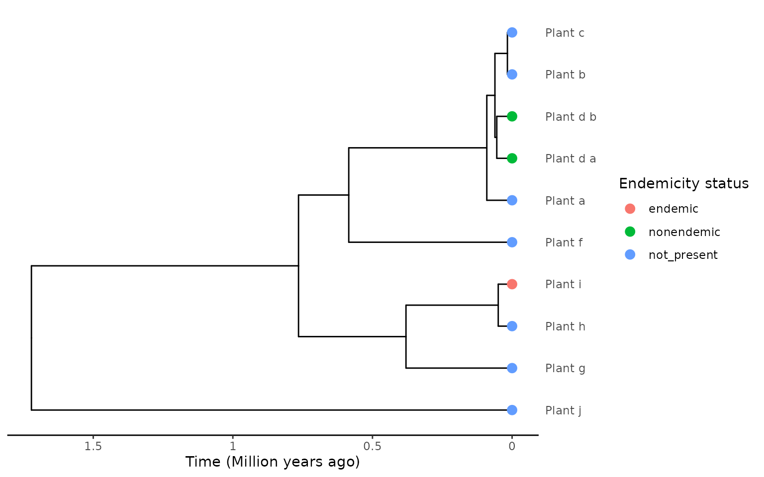

In this scenario we have a plant phylogeny with 9 species, and species “Plant_d” has two samples/tips in the tree. The samples are differentiated by the suffix labels: “_a” and “_b”.

Both “Plant_d” tips are labelled “nonendemic”, and this encoding is independent of where the samples for each tip were collected (species-dependent labelling), i.e. it is unknown if the non-endemic species have been sampled once on the island and once on the mainland, or twice on the island, or twice on the mainland. For the species-dependent encoding we assume that all tips are on the island and use the stem age of the species as the island colonisation time and the within species divergence as the minimum colonisation time when using the "min" extraction method.

There is one more island species in the phylogeny, “Plant_i”, which is endemic.

We can now extract the island community data using the "min" algorithm:

island_tbl <- extract_island_species(phylod = phylod, extraction_method = "min")
island_tbl
#> Class:  Island_tbl 
#>   clade_name     status missing_species   col_time col_max_age branching_times
#> 1    Plant_d nonendemic               0 0.06146596        TRUE              NA
#> 2    Plant_i    endemic               0 0.04960523       FALSE              NA
#>      min_age      species clade_type
#> 1 0.05480904 Plant_d_....          1
#> 2         NA      Plant_i          1

You can see that the extraction has successful extracted 2 island colonisations. The endemic “Plant_i” is extracted as per usual so we will not focus on that.

The “Plant_d” species has been correctly extracted as a single non-endemic species with a colonisation time (col_time), a minimum age of colonisation (min_age) which is taken from the branching time between the two non-endemic tips on the island. The logic here being that it is parsimonious to assume that the species colonised the island once and diverged on the island, and therefore the divergence would have been after the colonisation, providing a minimum bound to the colonisation time. There are no branching times (branching_times is NA) because there are no species-level speciation events on the island, only divergence below the level of the species.

Scenario: geography-dependent endemicity encoding

endemicity_status <- c("not_present", "not_present", "not_present", 
                       "nonendemic", "not_present", "not_present",
                       "not_present", "not_present", "endemic", "not_present")
phylod <- phylobase::phylo4d(phylo, as.data.frame(endemicity_status))
plot_phylod(phylod)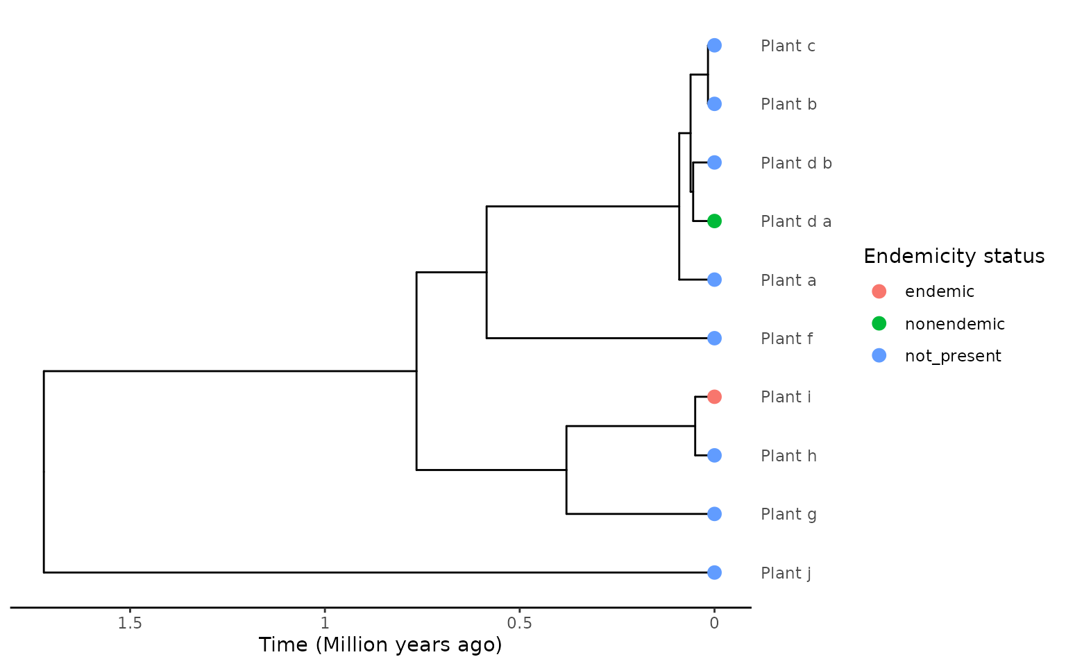

In this scenario we use the same phylogenetic data, but use a different labelling scheme. This time we use what we term geography-dependent labelling. This is where the tips in the phylogeny for multi-tip species are labelled according to where the sample was collected. So a sample from a non-endemic species sampled on the island would be labelled "nonendemic", but another sample from the same species from the mainland will be labelled "not_present".

The difference in the data with the first scenario is “Plant_d_b” is sampled from the mainland so it is now encoded as not being present on the island ("not_present").

island_tbl <- extract_island_species(phylod = phylod, extraction_method = "min")
island_tbl
#> Class:  Island_tbl 
#>   clade_name     status missing_species   col_time col_max_age branching_times
#> 1  Plant_d_a nonendemic               0 0.05480904       FALSE              NA
#> 2    Plant_i    endemic               0 0.04960523       FALSE              NA
#>   min_age   species clade_type
#> 1      NA Plant_d_a          1
#> 2      NA   Plant_i          1

We extract the island community data and see that again 2 colonisations are inferred, but this time there is not a min_age extracted as there are no subspecies divergences on the island.

Scenario: species-dependent endemicity encoding (endemics)

Revisiting the first scenario where we had multiple tips in the phylogeny from the same species, all labelled as non-endemic, independent of where the species sample came from, but this time the species is endemic to the island rather than non-endemic.

endemicity_status <- c("not_present", "not_present", "not_present", "endemic", 
                       "endemic", "not_present", "not_present", 
                       "not_present", "endemic", "not_present")
phylod <- phylobase::phylo4d(phylo, as.data.frame(endemicity_status))
plot_phylod(phylod)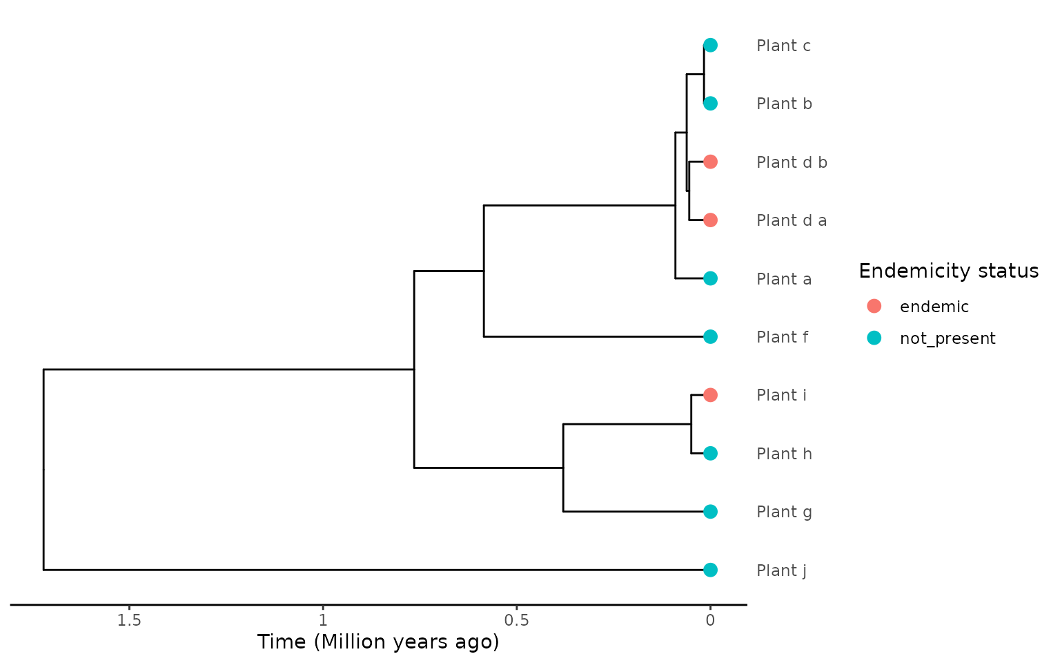

island_tbl <- extract_island_species(phylod = phylod, extraction_method = "min")
island_tbl
#> Class:  Island_tbl 
#>   clade_name  status missing_species   col_time col_max_age branching_times
#> 1    Plant_d endemic               0 0.06146596        TRUE              NA
#> 2    Plant_i endemic               0 0.04960523       FALSE              NA
#>      min_age      species clade_type
#> 1 0.05480904 Plant_d_....          1
#> 2         NA      Plant_i          1

The same extraction procedure, using the "min" algorithm, produces two endemic colonists. The multi-tip species is extracted with a colonisation time taken as the stem age of the species and minimum time of colonisation is taken from the within-species divergence (branching) time.

The extraction also works if you have more samples/tips per species. Here we increase the number of tips in the “Plant_d” species to 4.

phylobase::tipLabels(phylo) <- c("Plant_a", "Plant_d_a", "Plant_d_b",
                                 "Plant_d_c", "Plant_d_d", "Plant_b", "Plant_c",
                                 "Plant_e", "Plant_f", "Plant_g")
endemicity_status <- c("not_present", "endemic", "endemic", "endemic", 
                       "endemic", "not_present", "not_present", 
                       "not_present", "endemic", "not_present")
phylod <- phylobase::phylo4d(phylo, as.data.frame(endemicity_status))
plot_phylod(phylod)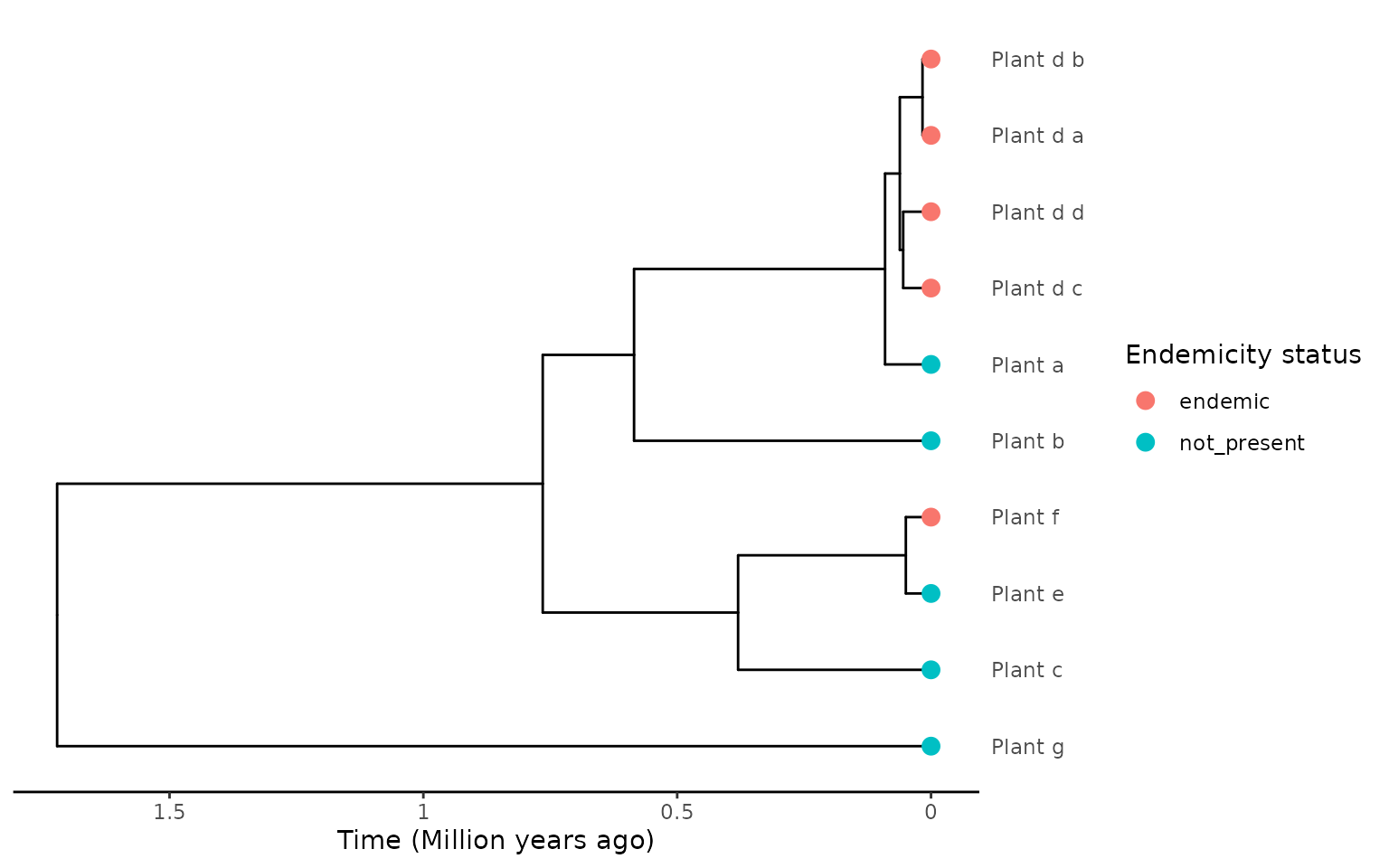

island_tbl <- extract_island_species(phylod = phylod, extraction_method = "min")
island_tbl
#> Class:  Island_tbl 
#>   clade_name  status missing_species   col_time col_max_age branching_times
#> 1    Plant_d endemic               0 0.09053720        TRUE              NA
#> 2    Plant_f endemic               0 0.04960523       FALSE              NA
#>      min_age      species clade_type
#> 1 0.06146596 Plant_d_....          1
#> 2         NA      Plant_f          1

The minimum age of colonisation in this case is the crown age of the 4 samples of the same species, with all species samples stored in the $species column.

Scenario: geography-dependent endemicity encoding (multiple island samples)

Lastly, we look once again at the endemicity encoding where island samples are labelled as endemic or non-endemic, and mainland samples are labelled not on the island (even if a non-endemic island species, geography-dependent labelling). This time with multiple samples from the island that are monophyletic.

In this scenario we look at a simple case of a single island species (“Plant_g”) in the tree, with 3 samples, 2 on the island (“Plant_g_island_a” and “Plant_g_island_b”) and 1 on the mainland (“Plant_g_mainland”).

phylobase::tipLabels(phylo) <- c("Plant_a", "Plant_b", "Plant_c", "Plant_d",
                                 "Plant_e", "Plant_f", "Plant_g_mainland",
                                 "Plant_g_island_b", "Plant_g_island_a", 
                                 "Plant_h")
endemicity_status <- c("not_present", "not_present", "not_present", 
                       "not_present", "not_present", "not_present", 
                       "not_present", "nonendemic", "nonendemic", 
                       "not_present")
phylod <- phylobase::phylo4d(phylo, as.data.frame(endemicity_status))
plot_phylod(phylod)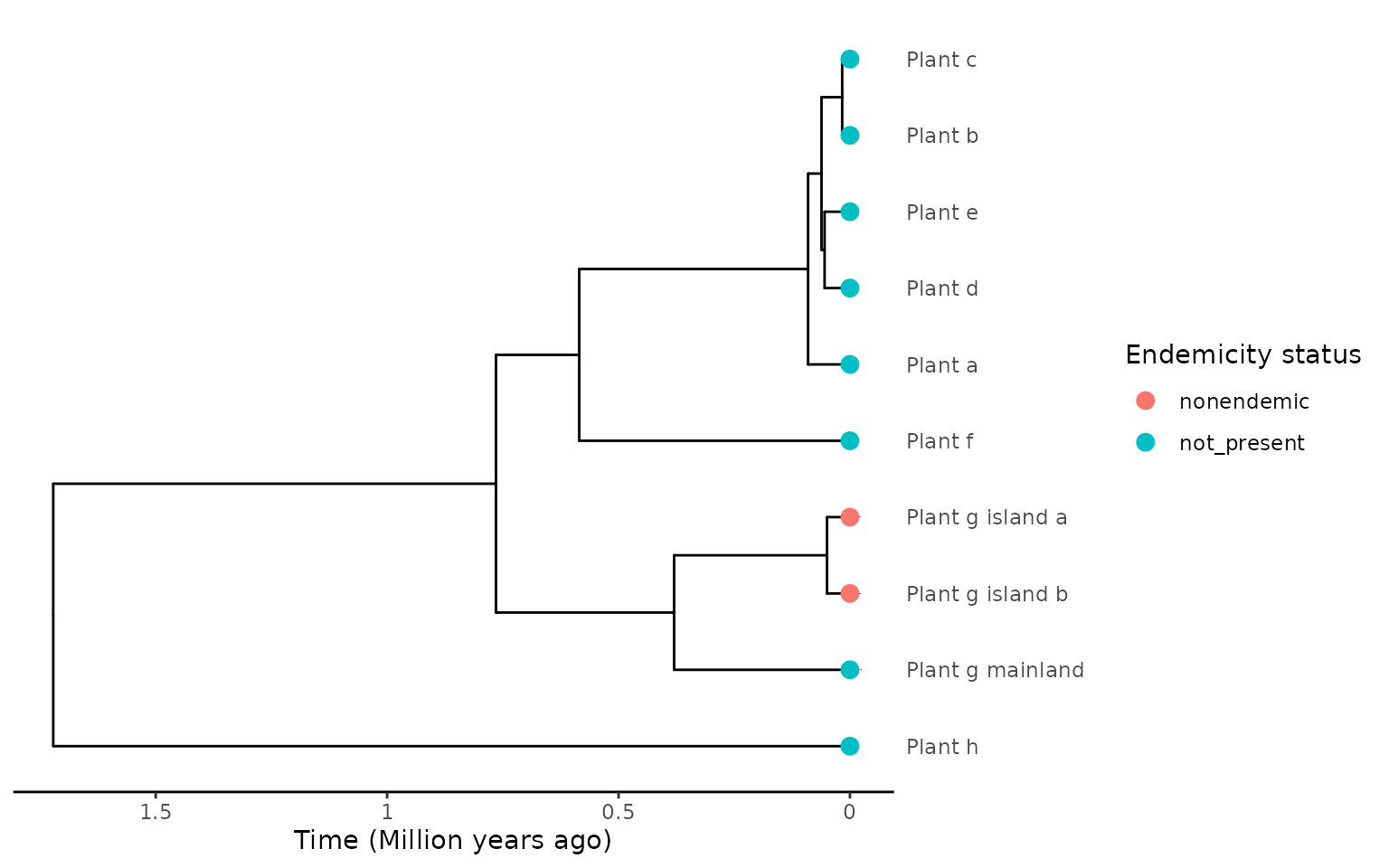

island_tbl <- extract_island_species(phylod = phylod, extraction_method = "min")
island_tbl
#> Class:  Island_tbl 
#>   clade_name     status missing_species  col_time col_max_age branching_times
#> 1    Plant_g nonendemic               0 0.3800341        TRUE              NA
#>      min_age      species clade_type
#> 1 0.04960523 Plant_g_....          1

The extracted island colonist has a colonisation time as the stem age of the island samples and the minimum colonisation time as the divergence of the island samples.