rm(list = ls())
library(ape)
library(DAISIEprep)
library(DAISIE)8 Answers
8.1 Example of how to extract data for Jamaica species from the Insula tree, add missing species, fit DAISIE models and run simulations.
A lot of the analyses here could be done in different ways, these are just options of how the exercise could be done.
8.1.1 Load required packages
8.1.2 Load tree
Insula_tree <- read.nexus("data/Insula.tre")Visualise tree (easier to use Figtree!)
plot(Insula_tree)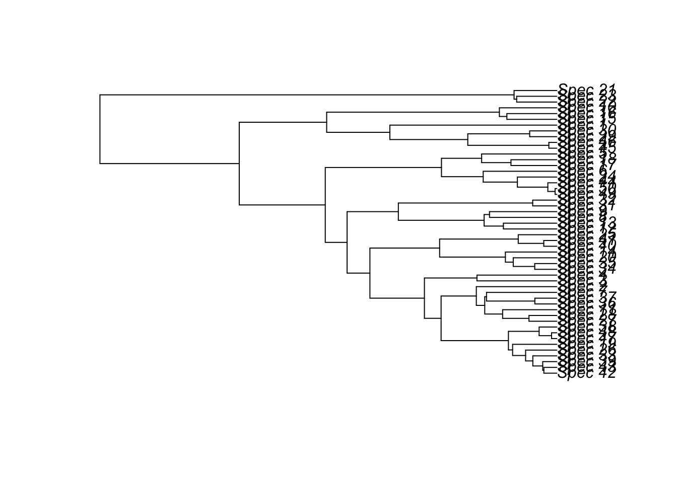
8.2 Prepare data using DAISIEprep
Look in the checklist to see which species occur on Jamaica. Specify tips corresponding to Jamaica species by specifying that they are endemic and/or non-endemic to the island:
island_species <- data.frame(
  tip_labels = c("Spec_29",
                 "Spec_48",
                 "Spec_47",
                 "Spec_38",
                 "Spec_43",
                 "Spec_42",
                 "Spec_39",
                 "Spec_33",
                 "Spec_26",
                 "Spec_19",
                 "Spec_41",
                 "Spec_40",
                 "Spec_25",
                 "Spec_9",
                 "Spec_24")
  ,
  tip_endemicity_status = c(rep("endemic",14),"nonendemic"))
Assign island endemicity status to all species in the dataset (including the non-Jamaican species)
endemicity_status <- create_endemicity_status(
  phylo = Insula_tree,
  island_species = island_species
)
Add endemicity status to the phylogeny
phylod <- phylobase::phylo4d(Insula_tree, endemicity_status)Visualize this on the tree
plot_phylod(phylod = phylod)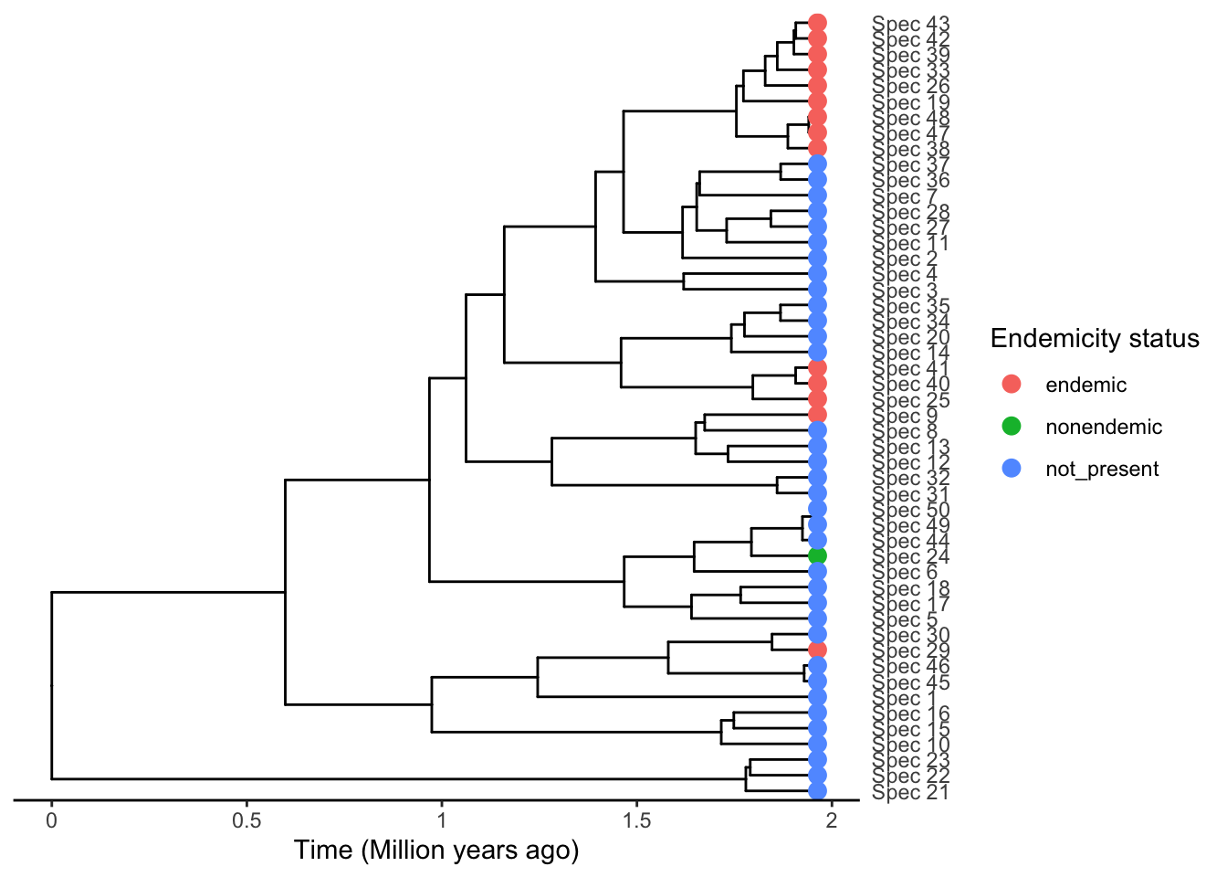
Extract data from the phylogeny using the min algorithm
island_tbl_min <- extract_island_species(
  phylod = phylod,
  extraction_method = "min"
)
island_tbl_min
Class: Island_tbl
clade_name status missing_species col_time col_max_age branching_times
1 Spec_9 endemic 0 0.2892541 FALSE NA
2 Spec_19 endemic 0 0.4972437 FALSE 0.207998....
3 Spec_24 nonendemic 0 0.1694692 FALSE NA
4 Spec_25 endemic 0 0.5035954 FALSE 0.165789....
5 Spec_29 endemic 0 0.1166231 FALSE NA
min_age species clade_type
1 NA Spec_9 1
2 NA Spec_19,.... 1
3 NA Spec_24 1
4 NA Spec_25,.... 1
5 NA Spec_29 1Extract data from the phylogeny using the ancestral state algorithm
phylod <- add_asr_node_states(phylod = phylod, asr_method = "mk")
plot_phylod(phylod = phylod)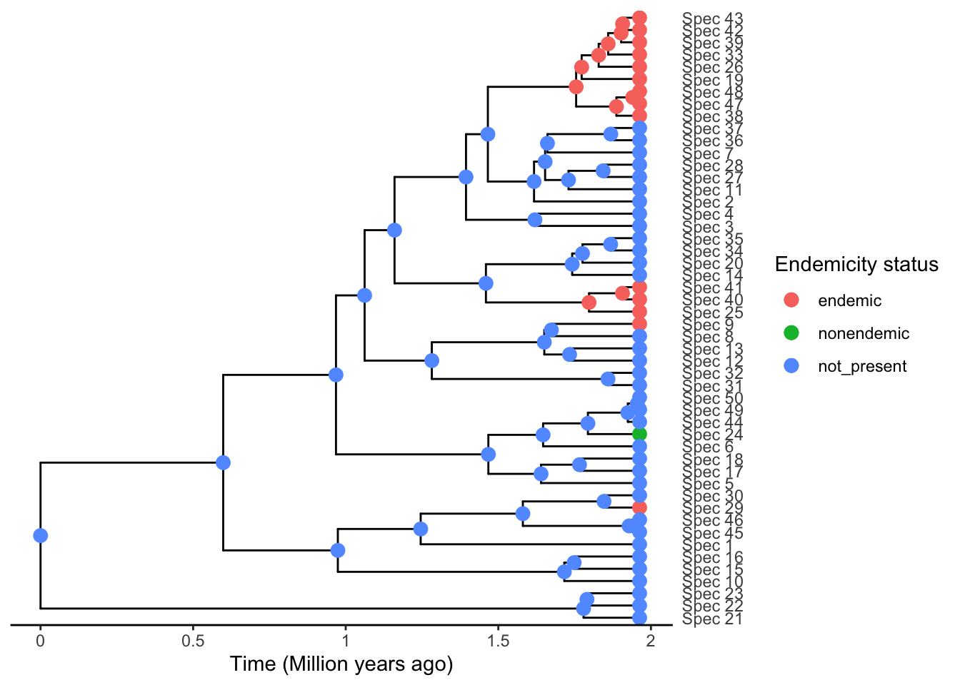
island_tbl_asr <- extract_island_species(
  phylod = phylod,
  extraction_method = "asr"
)
island_tbl_asr
Class: Island_tbl
clade_name status missing_species col_time col_max_age branching_times
1 Spec_9 endemic 0 0.2892541 FALSE NA
2 Spec_19 endemic 0 0.4972437 FALSE 0.207998....
3 Spec_24 nonendemic 0 0.1694692 FALSE NA
4 Spec_25 endemic 0 0.5035954 FALSE 0.165789....
5 Spec_29 endemic 0 0.1166231 FALSE NA
min_age species clade_type
1 NA Spec_9 1
2 NA Spec_19,.... 1
3 NA Spec_24 1
4 NA Spec_25,.... 1
5 NA Spec_29 1Compare 2 options:
all.equal(island_tbl_min,island_tbl_asr)[1] TRUEAs you can see, the results of the 2 extractions (min and asr) are exactly the same in this case, so we can use either for the subsequent analyses.
8.2.1 Add missing species
Add missing species “Spec_51”, which is not closely related to any species
island_tbl <- island_tbl_min
island_tbl <- add_island_colonist(
  island_tbl = island_tbl,
  clade_name = "Spec_51",
  status = "endemic",
  missing_species = 0,
  col_time = NA_real_,
  col_max_age = FALSE,
  branching_times = NA_real_,
  min_age = NA_real_,
  clade_type = 1,
  species = "Spec_51"
)
An alternative is to set the colonisation time to be younger than the mainland clade it is related to, by setting col_time to the age you choose and setting col_max_age=TRUE to tell DAISIE that is a maximum age for colonisation.
Add missing species Spec_52, closely related to Spec_42
island_tbl <- add_missing_species(
  island_tbl = island_tbl,
  num_missing_species = 1,
  species_to_add_to = "Spec_42"
)
Create DAISIE datalist
insula_data_list <- create_daisie_data(
  data = island_tbl,
  island_age = 5,
  num_mainland_species = 1000,
  precise_col_time = TRUE
)
8.3 Fit DAISIE models to data
Fit model with 5 parameters
M1 <- DAISIE_ML(
  datalist = insula_data_list,
  initparsopt = c(1.5,1.1,20,0.009,1.1),
  ddmodel = 11,
  idparsopt = 1:5,
  parsfix = NULL,
  idparsfix = NULL
)
M1
lambda_c mu K gamma lambda_a loglik df conv
1 5.859948 7.770723 3707849 0.02505749 3.234032 -37.10764 5 0Fit model with no carrying capacity
M2 <- DAISIE_ML(
  datalist = insula_data_list,
  initparsopt = c(1.5,1.1,0.009,1.1),
  idparsopt = c(1,2,4,5),
  parsfix = Inf,
  idparsfix = 3,
  ddmodel=0
)
M2
lambda_c mu K gamma lambda_a loglik df conv
1 5.901964 7.820509 Inf 0.02522255 3.198683 -37.10743 4 0Fit model with no anagenesis (optional)
M3 <- DAISIE_ML(
  datalist = insula_data_list,
  initparsopt = c(1.5,1.1,0.009),
  idparsopt = c(1,2,4),
  parsfix = c(Inf,0),
  idparsfix = c(3,5),
  ddmodel=0
)
M3
lambda_c mu K gamma lambda_a loglik df conv
1 6.740009 8.743373 Inf 0.02747074 0 -37.30009 3 0Save model results in a table
model_results <- rbind(M1,M2,M3)
model_results
lambda_c mu K gamma lambda_a loglik df conv
1 5.859948 7.770723 3707849 0.02505749 3.234032 -37.10764 5 0
2 5.901964 7.820509 Inf 0.02522255 3.198683 -37.10743 4 0
3 6.740009 8.743373 Inf 0.02747074 0.000000 -37.30009 3 0Create AIC function for model comparison
AIC_compare <- function(LogLik,k){
  aic <- (2 * k) - (2 * LogLik)
  return(aic)
}
Compute AIC for all the models
AICs <- AIC_compare(c(M1$loglik,M2$loglik,M3$loglik),c(M1$df,M2$df,M3$df))
names(AICs) <- c('M1','M2','M3')
AICs
M1 M2 M3
84.21527 82.21486 80.60018 In this case, the preferred model is M3.
8.4 Simulate islands based on parameters from preferred model
Run simulations
Insula_sims <- DAISIE_sim(
  time = 5,
  M = 1000,
  pars = as.numeric(M3[1:5]),
  replicates = 100,
  verbose = 1,
  plot_sims = FALSE)
Plot simulations
DAISIE_plot_sims(Insula_sims)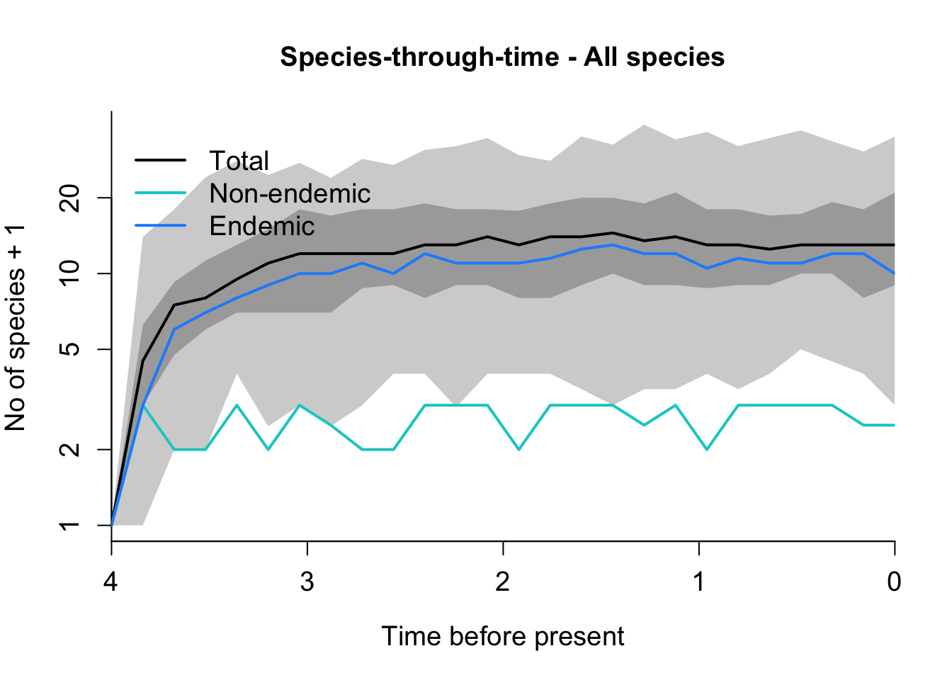
It looks like Insula diversity in the island of Jamaica is at a dynamic equilibrium.
To answer the last question, play around with different parameter settings in the simulation code. Be creative.