5 DAISIEprep

Author

Luis Valente, Joshua W. Lambert, Lizzie Roeble

5.1 Using DAISIEprep pack to extract and format data

In this part of the practical, the main features of DAISIEprep are explained. DAISIEprep (Lambert et al. 2023) is an R package that facilitates formatting of data for subsequent use in DAISIE.

A typical DAISIEprep pipeline is as follows:

Identify island colonisation events for the taxonomic group of interest from time-calibrated phylogenetic trees
Assign an island endemicity status (endemic, non-endemic, not present) to each of the species
Automatically extract times of colonisation of the island and diversification within the island from the phylogenies
Add any missing species
Format data for DAISIE.

The DAISIEprep tutorial is divided into the following sections:

Single Phylogeny example - Using a simulated phylogeny including island and non-island species, learn how to extract and format island data for running DAISIE.
Adding missing species - Learn how to add missing species, lineages, etc, to your DAISIE data list.
Prepare object for analyses in DAISIE

5.2 Single Phylogeny Example

In this section we demonstrate a simple example of extracting and formatting data from a single phylogeny. We use a simulated phylogeny, which facilitates explaining how the data is structured.

5.2.1 Load the required packages:

library(DAISIEprep)
library(ape)

5.2.2 Simulate example phylogeny

We now simulate a phylogeny using the package ape.

set.seed(
  4,
  kind = "Mersenne-Twister",
  normal.kind = "Inversion",
  sample.kind = "Rejection"
)
phylo <- ape::rcoal(10)

Important: DAISIEprep requires the tip labels (taxon names) in the phylogeny to be formatted as genus name and species name separated by an underscore (e.g. “Canis_lupus”, “Species_1”).

Here we add tip labels (representing our species) to the simulated phylogeny. In this case, all taxa sampled are different plant species from the same genus.

phylo$tip.label <- c("Plant_a", "Plant_b", "Plant_c", "Plant_d", "Plant_e",
                     "Plant_f", "Plant_g", "Plant_h", "Plant_i", "Plant_j")

Then we convert the phylogeny to a phylo4 class, defined in the package phylobase. This allows users to easily work with data for each tip in the phylogeny, for example whether they are endemic to the island or not.

phylo <- phylobase::phylo4(phylo)
phylobase::plot(phylo)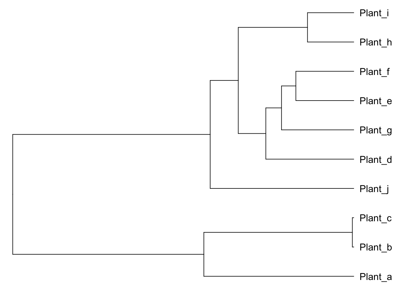

Now we have a phylogeny in the phylo4 format to which we can easily append data.

5.2.3 Add distribution information to the tips of the tree

Specify tips corresponding to species from your focal island by specifying that they are endemic and/or non-endemic to the island. In the example below, species Plant_h is found on the island but it not endemic, and species Plant_f and Plant_e are found on the island and are endemic to the island. All other species on the phylogeny are NOT present on the island.

island_species <- data.frame(
  tip_labels = c("Plant_h",
                 "Plant_f",
                 "Plant_e")
  ,
  tip_endemicity_status = c("nonendemic","endemic","endemic"))

Now that we know which species are present on the island, we can assign an endemicity status to all the species in the phylogeny.

endemicity_status <- create_endemicity_status(
  phylo = phylo,
  island_species = island_species
)

And append this information to the phylogeny object:

phylod <- phylobase::phylo4d(phylo, endemicity_status)

We can now visualise our phylogeny with the island endemicity statuses plotted at the tips. This uses the ggtree and ggplot2 packages.

plot_phylod(phylod = phylod)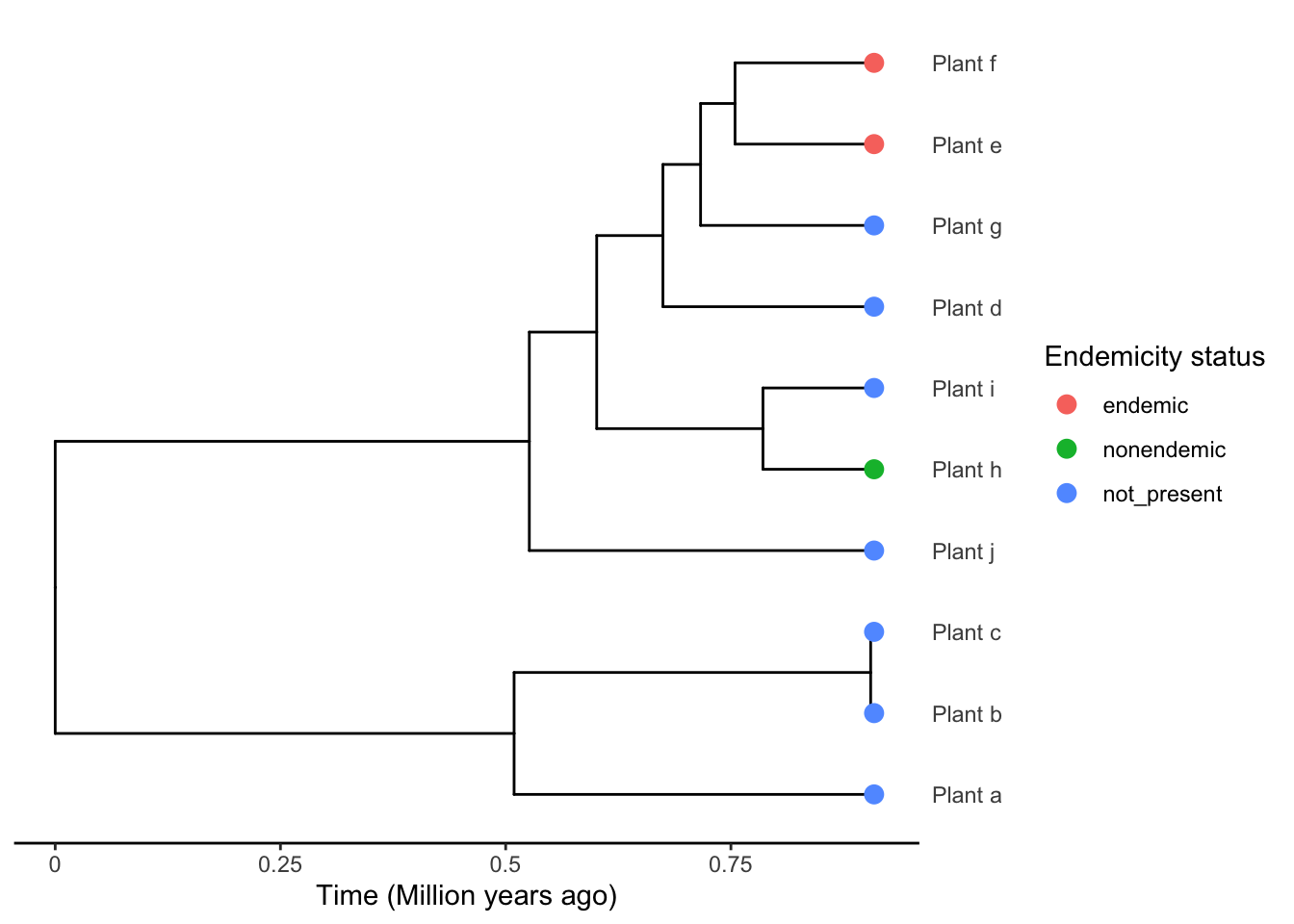

As you can see, in the example phylogeny, there appear to be 2 separate colonisation events of the island - one which has led to species Plant_f and Plant_e and other that has led to the non-endemic species Plant_h.

5.2.4 Extract data using DAISIEprep

Now that we can see the tips that are present on the island, we can extract them to form our island community data set that can be used in the DAISIE R package to fit likelihood models of island colonisation and diversification.

Before we extract species, we first create an object to store all of the island colonists’ information. This uses the island_tbl class introduced in this package (DAISIEprep). This island_tbl object can then easily be converted to a DAISIE data list using the function create_daisie_data (more information on this below).

island_tbl <- island_tbl()
island_tbl
#> Class:  Island_tbl 
#> [1] clade_name      status          missing_species col_time       
#> [5] col_max_age     branching_times min_age         species        
#> [9] clade_type     
#> <0 rows> (or 0-length row.names)

We can see that this is an object containing an empty data frame. In order to fill this data frame with information on the island colonisation and diversification events we can run:

island_tbl_min <- extract_island_species(
  phylod = phylod,
  extraction_method = "min"
)
island_tbl_min
#> Class:  Island_tbl 
#>   clade_name     status missing_species  col_time col_max_age branching_times
#> 1    Plant_e    endemic               0 0.1925924       FALSE    0.154371....
#> 2    Plant_h nonendemic               0 0.1233674       FALSE              NA
#>   min_age      species clade_type
#> 1      NA Plant_e,....          1
#> 2      NA      Plant_h          1

The function extract_island_species() is the main function in DAISIEprep to extract data from the phylogeny. In the example above, we used the “min” extraction algorithm. The “min” algorithm extracts island community data assuming no back-colonisation from the island to the mainland. Each row in the island_tbl corresponds to a separate colonisation of the island. In this case, two colonist lineages were correctly identified using the ‘min’ extraction algorithm, one endemic and another non-endemic. Each row in the table corresponds to one colonisation event.

However, if back-colonisation is frequent (for example, one species within a large endemic island radiation colonised another island or mainland), we recommend using the “asr” algorithm, which extracts the most likely colonisations inferred in an ancestral area reconstruction. To use the “asr” algorithm, we first need to know the probability of the ancestors of the island species being present on the island to determine the time of colonisation. To do this, we can fit one of many ancestral state reconstruction methods. Here we use the “mk” model (which uses a continuous-time markov model to reconstruct ancestral states), as it is a simple method that should prove reliable for reconstructing the ancestral species areas (i.e. on the island or not on the island) for most cases. First, we translate our extant species endemicity status to a numeric representation of whether that species is on the island.

phylod <- add_asr_node_states(phylod = phylod, asr_method = "mk")

Now we can plot the phylogeny, which this time includes the node labels for the presence/absence on the island in ancestral nodes.

plot_phylod(phylod = phylod)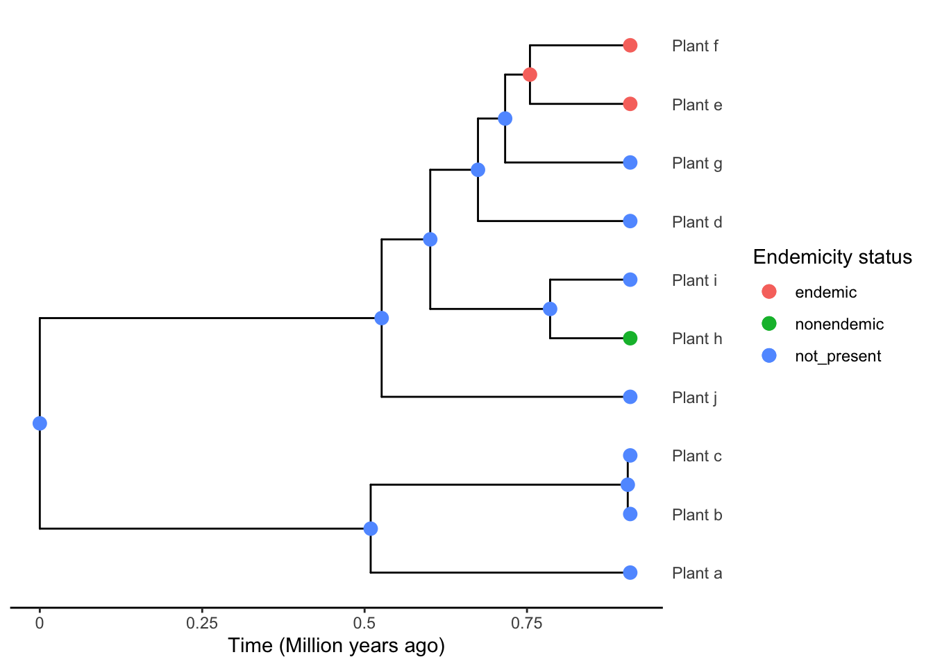

Sidenote (optional): if you are wondering what the probabilities are at each node and whether this should influence your decision to pick a preference for island or mainland when the likelihoods for each state are equal, we can plot the probabilities at the nodes to visualise the ancestral state reconstruction using plot_phylod(phylod = phylod, node_pies = TRUE).

Now we can extract island colonisation and diversification times from the phylogeny with asr using the reconstructed ancestral states of island presence/absence.

island_tbl_asr <- extract_island_species(
  phylod = phylod,
  extraction_method = "asr"
)

island_tbl_asr
#> Class:  Island_tbl 
#>   clade_name     status missing_species  col_time col_max_age branching_times
#> 1    Plant_e    endemic               0 0.1925924       FALSE    0.154371....
#> 2    Plant_h nonendemic               0 0.1233674       FALSE              NA
#>   min_age      species clade_type
#> 1      NA Plant_e,....          1
#> 2      NA      Plant_h          1

By comparing island_tbl_min and island_tbl_asr you can see the differences in the 2 extraction methods.

all.equal(island_tbl_min,island_tbl_asr)
#> [1] TRUE

In this case, the results using “asr” and “min” are exactly the same. For the purposes of this practical, we will proceed with the results from “asr” (island_tbl_asr). For convenience, let’s rename the object to island_tbl.

island_tbl<-island_tbl_asr

You can visualize the contents of the island_tbl object to try and figure out what they mean.

View(island_tbl)

For example, the code below shows you the names of the species included in each lineage:

island_tbl@island_tbl$species
#> [[1]]
#> [1] "Plant_e" "Plant_f"
#> 
#> [[2]]
#> [1] "Plant_h"

5.3 Adding missing species

It is often the case that phylogenetic data is not available for some island species or even for entire lineages present in the island community. But we can still include these species in our DAISIE analyses using DAISIEprep. This section is about the tools that DAISIEprep provides in order to handle missing data, and generally to handle species that are missing and need to be input into the data manually.

For this section, as with the previous section, the core data structure we are going to work with is the island_tbl. We will use the island_tbl for the example plant dataset produced in the last section.

5.3.1 Adding missing species to an island clade that has been sampled in the phylogeny

This option is for cases in which a clade has been sampled in the phylogeny, and at least 1 colonisation or 1 branching time is available in the datalist, but 1 or more species from that clade were not sampled. For this example, we imagine that 2 species have not been sampled, and that we want to add them as missing species to the lineage containing species “Plant_e” that is sampled in the phylogeny. To assign two missing species to this clade we use the function add_missing_species() The argument species_to_add_to uses a representative sampled species from that island clade to work out which colonist in the island_tbl to assign the specified number of missing species (num_missing_species) to. You can find out which species are already sampled in each lineage using:

island_tbl@island_tbl$species
#> [[1]]
#> [1] "Plant_e" "Plant_f"
#> 
#> [[2]]
#> [1] "Plant_h"

Now run the code:

island_tbl <- add_missing_species(
  island_tbl = island_tbl,
  # num_missing_species equals total species missing
  num_missing_species = 2,
  # name of a sampled species you want to "add" the missing to
  # it can be any in the clade
  species_to_add_to = "Plant_e"
)

The new island table now has missing species added to the lineage we wanted to:

island_tbl@island_tbl$missing_species
#> [1] 2 0

With the new missing species added to the island_tbl we can repeat the conversion steps above using create_daisie_data() to produce data accepted by the DAISIE model.

data_list <- create_daisie_data(
  data = island_tbl,
  island_age = 12,
  num_mainland_species = 100,
  precise_col_time = TRUE
)

5.3.2 Adding an entire lineage when a phylogeny is not available for the lineage.

For cases when the missing species belong to a lineage that has not been sampled in the phylogeny. Assuming we did not have any phylogenetic data or colonisation time estimate for the island clade, we can insert species as missing and specify them as a separate lineage. Because no colonisation and branching times are known for this lineage, when this lineage later gets processed by the DAISIE inference model it will be assumed it colonised the island any time between the island’s formation and the present.

The input needed are:

island_tbl to add to an existing island_tbl
clade_name a name to represent the new clade addeed, can either be a specific species from the clade or a genus name, or another name that represent those species
status either “endemic” or “nonendemic”
species a vector of species names contained within colonist (if applicable)
missing_species In the case of a lineage with just 1 species (i.e. not an island radiation) the number of missing species is zero, as by adding the colonist it already counts as one automatically. In the case of an island clade of more than one species, the number of missing species in this case should be n-1.

Example for adding lineage with 1 species:

island_tbl <- add_island_colonist(
  island_tbl = island_tbl,
  clade_name = "Plant_y",
  status = "endemic",
  # clade with just 1 species, missing_species = 0
  # because adding the lineage already counts as 1
  missing_species = 0,
  col_time = NA_real_,
  col_max_age = FALSE,
  branching_times = NA_real_,
  min_age = NA_real_,
  clade_type = 1,
  species = "Plant_a"
)

Example for adding lineage with 5 species (“Plant_a”, “Plant_b”, “Plant_c”, “Plant_d”, “Plant_e”) to a lineage called “Plant_radiation”

island_tbl <- add_island_colonist(
  island_tbl = island_tbl,
  clade_name = "Plant_radiation",
  status = "endemic",
  # the total species is 5 and all are missing
  # but we add missing_species = 4 because
  # adding the lineage already counts as 1
  missing_species = 4,
  col_time = NA_real_,
  col_max_age = FALSE,
  branching_times = NA_real_,
  min_age = NA_real_,
  clade_type = 1,
  species = c("Plant_a", "Plant_b", "Plant_c",
              "Plant_d", "Plant_e")
)

5.4 Prepare object for analyses in DAISIE

Convert to data object to be used in DAISIE

Now that we have the island_tbl we can convert this to the DAISIE data list to be used by the DAISIE inference model. To convert to the DAISIE data list (i.e. the input data of the DAISIE inference model) we use create_daisie_data(), providing the island_tbl as input. We also need to specify:

The age of the island or archipelago. Here we use an island age of twelve million years (island_age = 12).
Whether the colonisation times extracted from the phylogenetic data should be considered precise (precise_col_time = TRUE). We will not discuss the details of this here, but briefly by setting this to TRUE the data will tell the DAISIE model that the colonisation times are known without error. Setting precise_col_time = FALSE will change tell the DAISIE model that the colonisation time is uncertain and should interpret this as the upper limit to the time of colonisation and integrate over the uncertainty between this point and either the present time or to the first branching point (either speciation or divergence into subspecies).
The number of species in the mainland source pool. Here we set it to 100 (num_mainland_species = 100). This will be used to calculate the number of species that could have potentially colonised the island but have not. When we refer to the mainland pool, this does not necessarily have to be a continent, it could be a different island if the source of species immigrating to an island is largely from another nearby island (a possible example of this could be Madagascar being the source of species colonising Comoros). This information is used by the DAISIE model to calculate the colonisation rate of the island.

data_list <- create_daisie_data(
  data = island_tbl,
  island_age = 12,
  num_mainland_species = 100,
  precise_col_time = TRUE
)

Below we show two elements of the DAISIE data list produced. The first element data_list[[1]] in every DAISIE data list is the island community metadata, containing the island age and the number of species in the mainland pool that did not leave descendants on the island at the present day. This is important information for DAISIE inference, as it is possible some mainland species colonised the island but went extinct leaving no trace of their island presence.

data_list[[1]]
#> $island_age
#> [1] 12
#> 
#> $not_present
#> [1] 96

Next is the first element containing information on island colonists (every element data_list[[x]] in the list after the metadata contains information on individual island colonists). This contains the name of the colonist, the number of missing species, and the branching times, which is a vector containing the age of the island, the colonisation time and the times of any cladogenesis events. Confusingly, it may be that the branching times vector contains no branching times: when there are only two numbers in the vector these are the island age followed by the colonisation time. Then there is the stac, which stands for status of colonist. This is a number which tells the DAISIE model how to identify the endemicity and colonisation uncertainty of the island colonist (these are explained here if you are interested). Lastly, the type1or2 defines which macroevolutionary regime an island colonist is in. By macroevolutionary regime we mean the set of rates of colonisation, speciation and extinction for that colonist. Most applications will assume all island clades have the same regime and thus all are assigned type 1. However, if there is a priori expectation that one clade significantly different from the rest, e.g. the Galápagos finches amongst the other terrestrial birds of the Galápagos archipelago this clade can be set to type 2.

data_list[[2]]
#> $colonist_name
#> [1] "Plant_e"
#> 
#> $branching_times
#> [1] 12.0000000  0.1925924  0.1543711
#> 
#> $stac
#> [1] 2
#> 
#> $missing_species
#> [1] 2
#> 
#> $type1or2
#> [1] 1

This datalist is now ready to be used in the DAISIE maximum likelihood inference model from the R package DAISIE.

End of the DAISIEprep tutorial!