5 Summary and error metrics visualisation

There is a range of plotting functions to visualise the summary metrics and error metrics (Section 4.3).

For the plotting of simulation summary and error metrics we need to load the results from multiple different mainland extinction scenarios.

analysis_results <- DAISIEmainland::read_analysis_results(
  data_folder_path = system.file(
    "/inst/book/data/param_sets/", 
    package = "DAISIEmainland"
  )
)

5.1 Simulation summary metrics

First we run the simulation. This is the same simulation as in the inference performance section (Section 4.1).

set.seed(
  1,
  kind = "Mersenne-Twister",
  normal.kind = "Inversion",
  sample.kind = "Rejection"
)

replicates <- 100

daisie_mainland_data <- DAISIEmainland::sim_island_with_mainland(
  total_time = 1,
  m = 100,
  island_pars = c(0.5, 02.5, 50, 0.01, 0.5),
  mainland_ex = 1.0,
  mainland_sample_prob = 1,
  mainland_sample_type = "complete",
  replicates = replicates,
  verbose = FALSE
)

The simulation summary metrics we can calculate for the ideal and empirical data are:

number of species on the island at the end of the simulation.
number of colonisation events to the island (that survived to the present) at the end of the simulation.

ideal_sim_num_spec <- DAISIEmainland::calc_num_spec(
  multi_daisie_data = daisie_mainland_data$ideal_multi_daisie_data
)

ideal_sim_num_spec
#>   [1] 120  94  89  76  63  91  93  81  58 135  95  78 118  93  97 115 109 128 142  73  71  55 109 102 123 134  93 103
#>  [29]  82  73 125  91  83  85 100 107  88  94  95 138 116  89  86 119  60  83 103  87 106 114  72 133 113  80 131  92
#>  [57]  95  81  91  79  66 120 107  69  91  80  71 138 101  99  78  52 173 125  83  76  78  59  94  98 104  68  81  80
#>  [85]  74  94 113  96  76 113  78  85  67 123  70  73  63 127 105  85

ideal_sim_num_col <- DAISIEmainland::calc_num_col(
  multi_daisie_data = daisie_mainland_data$ideal_multi_daisie_data
)

ideal_sim_num_col
#>   [1] 44 33 39 28 29 30 33 35 28 42 36 32 46 38 30 38 45 40 40 28 28 28 41 34 39 45 34 32 33 29 31 36 33 32 38 34 36 31
#>  [39] 29 41 43 34 36 34 24 30 33 28 42 37 24 37 43 33 45 35 27 37 37 28 29 40 36 30 31 32 27 48 40 47 30 22 41 38 37 27
#>  [77] 35 28 37 33 40 27 38 30 35 38 39 37 30 37 31 33 25 42 35 37 29 31 31 36

empirical_sim_num_spec <- DAISIEmainland::calc_num_spec(
  multi_daisie_data = daisie_mainland_data$empirical_multi_daisie_data
)

empirical_sim_num_spec
#>   [1] 120  94  89  76  63  91  93  81  58 135  95  78 118  93  97 115 109 128 142  73  71  55 109 102 123 134  93 103
#>  [29]  82  73 125  91  83  85 100 107  88  94  95 138 116  89  86 119  60  83 103  87 106 114  72 133 113  80 131  92
#>  [57]  95  81  91  79  66 120 107  69  91  80  71 138 101  99  78  52 173 125  83  76  78  59  94  98 104  68  81  80
#>  [85]  74  94 113  96  76 113  78  85  67 123  70  73  63 127 105  85

empirical_sim_num_col <- DAISIEmainland::calc_num_col(
  multi_daisie_data = daisie_mainland_data$empirical_multi_daisie_data
)

empirical_sim_num_col
#>   [1] 43 33 38 28 28 28 32 33 28 42 36 32 46 37 30 37 43 39 38 28 27 28 39 34 39 45 34 32 33 29 31 36 32 30 36 33 34 31
#>  [39] 29 40 41 32 36 33 24 29 32 28 40 34 23 36 42 33 44 35 27 35 36 28 28 40 35 30 30 32 27 44 40 44 29 22 40 38 37 25
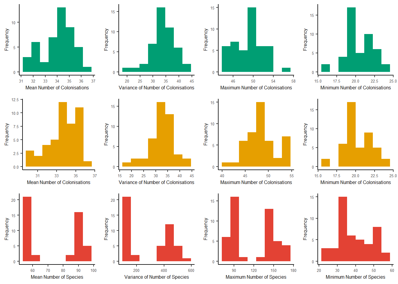
#>  [77] 34 27 35 33 39 26 38 30 35 37 39 37 29 37 30 33 25 42 35 36 29 31 30 35

We can plot the simulation summary metrics to view the mean, variance, maximum and minimum number of colonisations and number of species for the ideal and empirical data.

plot_sim_metrics(
  analysis_results = analysis_results, 
  output_file_path = NULL
)

5.2 Inference error metrics

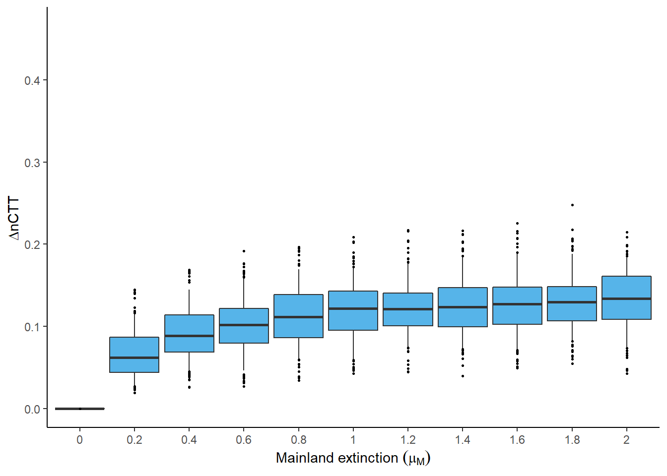
The error metrics were run for a range of mainland extinction rates. Then, the error metrics can be plotted across different rates to determine how the error varies with faster or slower mainland evolutionary dynamics.

Thus, plotting the \(\Delta\)CTT across mainland extinction rates between zero and two (per species per million years) is informative. As explained in Section 4.3 this metric is a comparison between the ideal and empirical data sets produced by the DAISIEmainland simulation.

plot_ctt_boxplot(
  analysis_results = analysis_results, 
  output_file_path = NULL,
  parameter = "mainland_ex"
)

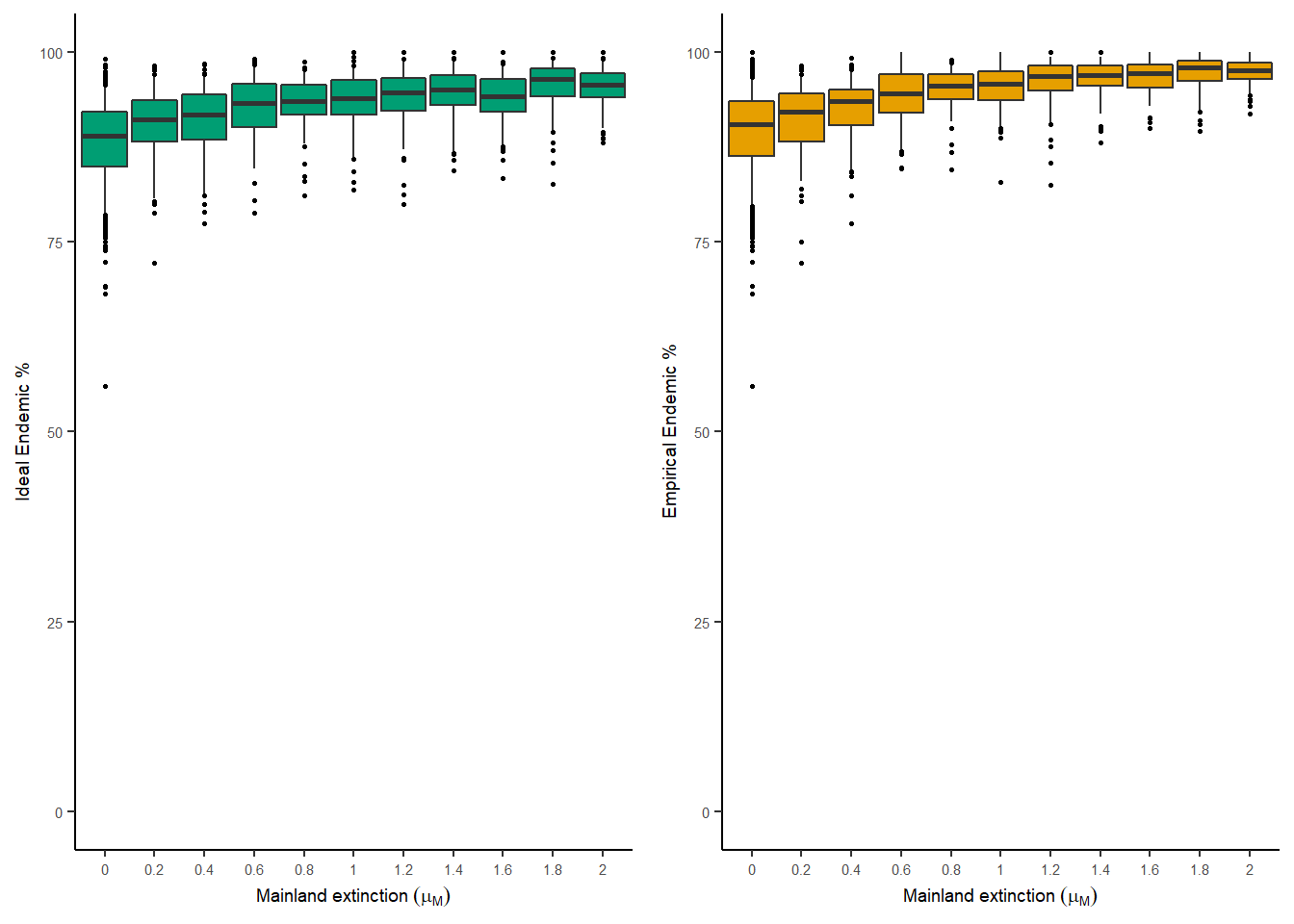
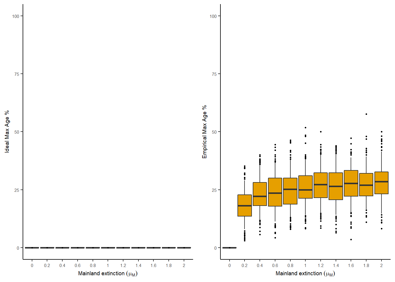
The percentage of endemics on the island at the end of the simulation and percentage of maximum age colonisation times can be plotted for different values of mainland extinction. Each of the boxplots below shows 100 island replicates. The left hand panel is for the data set with complete information (ideal) and the right hand panel is for the data set with incomplete information (empirical).

plot_endemics(
  analysis_results = analysis_results, 
  output_file_path = NULL, 
  parameter = "mainland_ex"
)

plot_max_age(
  analysis_results = analysis_results, 
  output_file_path = NULL, 
  parameter = "mainland_ex"
)

The plots shown in this chapter are not an exhaustive list available from the package. For example, error metrics can also be plotted across different values of mainland sampling probability by setting the parameter = "mainland_sample_prob" in the plotting functions. The script used to make the plots for the two manuscripts using this package can be found here and here.

4 Inference performance

6 References