In [1]:

# Define the x values for the plot
x <- seq(0, 10, length.out = 100)
shape_scale <- stats::dgamma(x = x, shape = 2, scale = 2)
shape_rate <- stats::dgamma(x = x, shape = 2, rate = 2)
plot(x, shape_rate, type = "l", col = "blue", lwd = 2, ylab = "Density", 
     xlab = "x", main = "Gamma Distribution")
lines(x, shape_scale, col = "red", lwd = 2)

meanlog_sdlog <- stats::dlnorm(x = x, meanlog = 0.5, sdlog = 0.5)
mean_sd <- stats::dlnorm(x = x, meanlog = 1.87, sdlog = 1)
plot(x, meanlog_sdlog, type = "l", col = "coral", lwd = 2, ylab = "Density", 
     xlab = "x", main = "Lognormal Distribution")
# Add the Gamma distribution with scale = 2
lines(x, mean_sd, col = "green", lwd = 2)

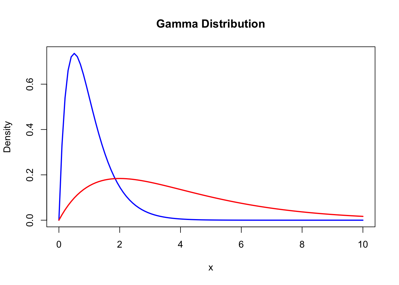
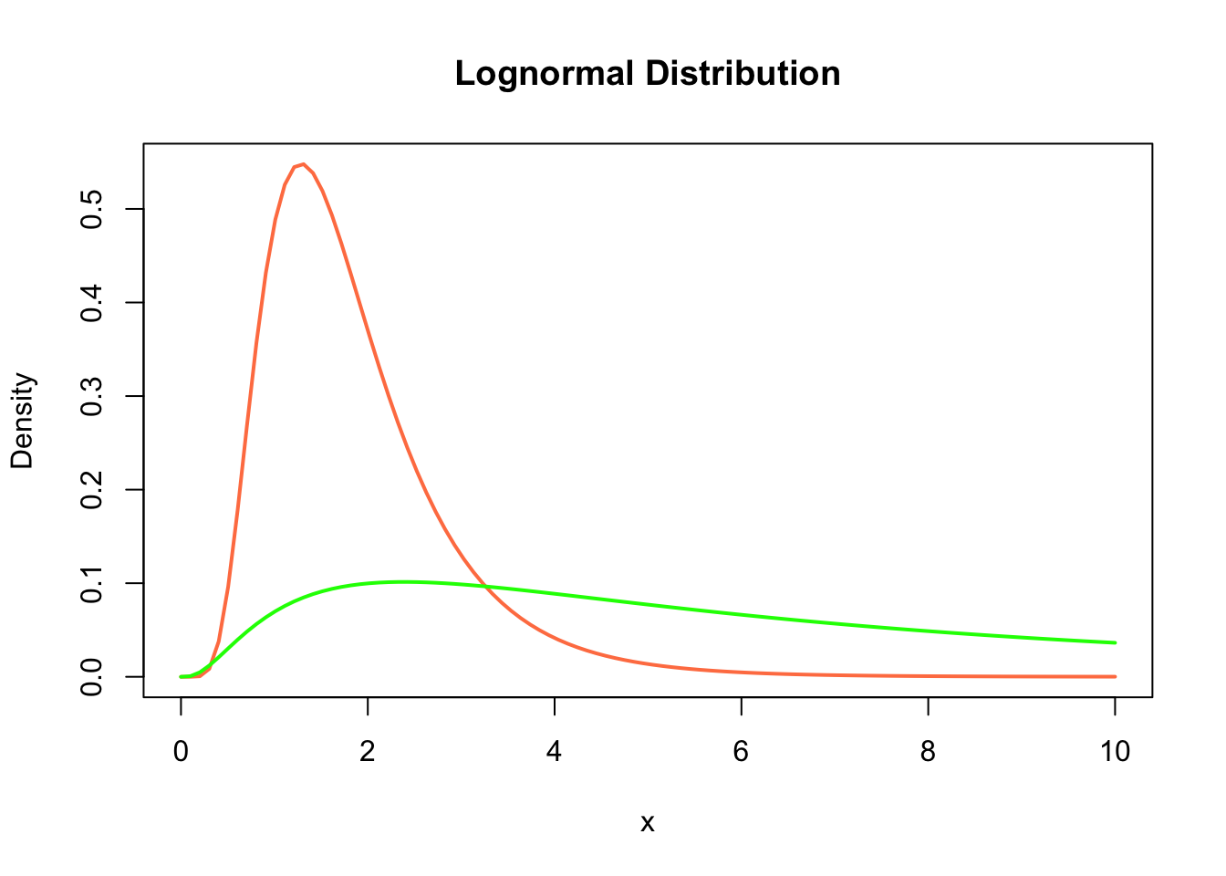
Differences in distributions when misinterpreting the estimated parameters. (a) Two gamma distributions, the blue shows a gamma distribution with shape (\(\alpha\)) and rate (\(\beta\)) of 2, the red shows a gamma distribution with shape (\(k\)) and scale (\(\theta\)) of 2. The rate is the reciprocal of the scale (\(\beta\) = 1/\(\theta\)), but it is clear from the left hand plot that misinterpreting the parameter leads to a vastly different distribution density. (b) Two lognormal distributions, the orange shows the density of a lognormal distribution with meanlog (\(\mu\)) and sdlog (\(\sigma\)) of 0.5, and the green with the meanlog and sdlog of 1.87 and 1.00, respectively (these values are the conversion from meanlog and sdlog into mean and standard deviation). Again showing how misinterpreting the parameters can lead to differences in epidemiological parameters.

Differences in distributions when misinterpreting the estimated parameters. (a) Two gamma distributions, the blue shows a gamma distribution with shape (\(\alpha\)) and rate (\(\beta\)) of 2, the red shows a gamma distribution with shape (\(k\)) and scale (\(\theta\)) of 2. The rate is the reciprocal of the scale (\(\beta\) = 1/\(\theta\)), but it is clear from the left hand plot that misinterpreting the parameter leads to a vastly different distribution density. (b) Two lognormal distributions, the orange shows the density of a lognormal distribution with meanlog (\(\mu\)) and sdlog (\(\sigma\)) of 0.5, and the green with the meanlog and sdlog of 1.87 and 1.00, respectively (these values are the conversion from meanlog and sdlog into mean and standard deviation). Again showing how misinterpreting the parameters can lead to differences in epidemiological parameters.